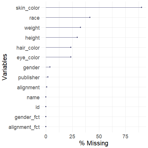
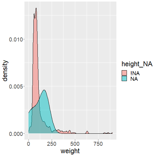
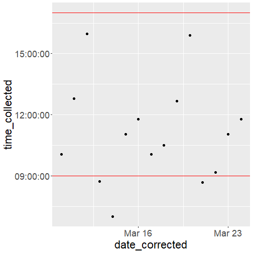
class: inverse background-image: url(../slides/images/better_data_cleaning_splash_slide_section_3.png) background-position: center background-size: contain --- class: inverse ## Outline 1. [Missing Data Profiling](#missingdata) 2. [Handling Dates](#dates) --- class: inverse names: missingdata ## Missing Data Missing data can be tricky and problematic, but profiling patterns of missingness in a dataset need not be. We will be using the following packages in this section. ```r install.packages(c("tidyverse","here","naniar")) ``` -- Don't forget to load the packages after the install is complete. ```r library(tidyverse) library(here) library(naniar) ``` --- class: inverse ## Missing Data: Load the Data ```r # Run the entire cleaning script to reproduce our cleaned version of the superhero data source(here("scripts","cleaning_script.R")) ``` ``` ## Parsed with column specification: ## cols( ## X1 = col_double(), ## name = col_character(), ## Gender = col_character(), ## `Eye color` = col_character(), ## Race = col_character(), ## `Hair color` = col_character(), ## Height = col_double(), ## Publisher = col_character(), ## `Skin color` = col_character(), ## Alignment = col_character(), ## Weight = col_double() ## ) ``` --- class: inverse ## Let's Take a Peak at the Data ```r # Take a peak inside to ensure that it was loaded correctly glimpse(data_superhero) ``` ``` ## Rows: 734 ## Columns: 13 ## $ id <dbl> 0, 1, 2, 3, 4, 5, 6, 7, 8, 9, 10, 11, 12, 13, 14... ## $ name <chr> "A-Bomb", "Abe Sapien", "Abin Sur", "Abomination... ## $ gender <chr> "male", "male", "male", "male", "male", "male", ... ## $ eye_color <chr> "yellow", "blue", "blue", "green", "blue", "blue... ## $ race <chr> "human", "icthyo sapien", "ungaran", "human / ra... ## $ hair_color <chr> "no hair", "no hair", "no hair", "no hair", "bla... ## $ height <dbl> 203, 191, 185, 203, NA, 193, NA, 185, 173, 178, ... ## $ publisher <chr> "marvel comics", "dark horse comics", "dc comics... ## $ skin_color <chr> NA, "blue", "red", NA, NA, NA, NA, NA, NA, NA, N... ## $ alignment <chr> "good", "good", "good", "bad", "bad", "bad", "go... ## $ weight <dbl> 441, 65, 90, 441, NA, 122, NA, 88, 61, 81, 104, ... ## $ gender_fct <fct> male, male, male, male, male, male, male, male, ... ## $ alignment_fct <fct> good, good, good, bad, bad, bad, good, good, goo... ``` --- class: inverse .hex-sticker[] ## Visualize Missingness by Column -- .pull-left[ ```r # generate missing data visualization by columns gg_miss_var(data_superhero, show_pct = TRUE) ``` ] .pull-right[ <!-- --> ] --- class: inverse ## Visualize Intersections of Missingness While understanding how much data is missing in each column is important information, when trying to find patterns of missingness you need to examine the intersections of missingness. -- In essence, we might want to know the percentage of our data which has missing `weight` and `height`. -- This could help us when we make assumptions about patterns of missingness. --- class: inverse .hex-sticker[] ## Creating an Upset Plot ```r gg_miss_upset(data_superhero, nsets = 5, nintersects = NA, text.scale = c(2,1,1,1,2,1.3)) ``` We need to specify the dataset we want to use, the number of sets (which variables) to include, and the number of interactions we want to examine. If you set the `ninteractions` arugment to `NA`, then all interactions using the given variables will be displayed. --- class: inverse,middle, center .hex-sticker[] <img src="Section_3_files/figure-html/unnamed-chunk-7-1.png" width="750px" height="550px" /> --- class: inverse .hex-sticker[] ## Shadow Matrix A handy way to examine conditional missingness is to construct a shadow matrix [(Swayne and Buja, 1998)](https://www.researchgate.net/publication/2758672_Missing_Data_in_Interactive_High-Dimensional_Data_Visualization). This matrix has the same dimensions as the original dataset, but each column now has a parallel column which tracks the missingness of its partner. There are two ways of quickly constructing the shadow matrix: one way creates the matrix as a new dataset, the other appends the shadow matrix to the original dataset column-wise. ```r # create a shadow matrix of the superhero dataset as_shadow(data_superhero) # add the shadow matrix to the side of the superhero dataset bind_shadow(data_superhero) ``` --- class: inverse .hex-sticker[] ## Shadow Matrix: Profiling .pull-left[ ```r data_superhero %>% bind_shadow() %>% ggplot(aes(x = weight, fill = height_NA)) + geom_density(alpha = .5) ``` * Start with the superhero dataset, then ... * append the shadow matrix, then ... * construct a canvas using weight on the x-axis, and fill by using whether height is missing or not, then ... * generate a density plot with some transparency ] .pull-right[ <!-- --> ] --- class: inverse name: dates ## Working With Dates, Times, and Date-Times -- Dealing with dates can be tricky as there are many ways to write a date. I recommend changing your dates to align with the [ISO 8601](https://en.wikipedia.org/wiki/ISO_8601). The general principle behind this standard is ordering the date/time from the largest units to the smallest units. Adhering to this standard makes it clear how your data is stored and makes it easier to use. * 2020/03/04: is this March 4th, 2020; or April 3rd, 2020? * 20/03/05: is this March 20th, 2005; or June 3rd, 2020? Unless you document how the date is stored, only you will know the correct date. ??? The lubridate package has many handy function for managing three kinds of data: * date-time: which is stored as the number of seconds since 1970-01-01 00:00:00 UTC * date: which is stored as the number of days since 1970-01-01 * time: which is stored as the number of seconds since 00:00:00 --- class: inverse .hex-sticker[] ## Lubridate Let's try an example. This fictitious data was "collected" in March of 2020 across two different collection sites (A and B). We can start by loading the "date_time_data.csv" file and taking a peak. ```r library(lubridate) ``` ```r data_dates <- read_csv(here("data", "date_time_data.csv")) ``` ``` ## Parsed with column specification: ## cols( ## id = col_double(), ## date = col_character(), ## time_collected = col_time(format = ""), ## site = col_character() ## ) ``` --- .hex-sticker[] ## Lubridate <div id="htmlwidget-e2caca0304fb6017e73c" style="width:100%;height:auto;" class="datatables html-widget"></div> <script type="application/json" data-for="htmlwidget-e2caca0304fb6017e73c">{"x":{"filter":"none","fillContainer":false,"data":[["1","2","3","4","5","6","7","8","9","10","11","12","13","14","15"],[1,2,3,4,5,6,7,8,9,10,11,12,13,14,15],["20-03-10","20-03-11","20-03-12","20-03-13","20-03-14","20-03-15","20-03-16","17-3-20","18-3-20","19-3-20","20-3-20","21-3-20","22-3-21","23-3-20","24-3-20"],["10:03:00","12:47:00","15:59:00","08:43:00","07:00:00","11:03:00","11:47:00","10:03:00","10:30:00","12:40:00","15:54:00","08:40:00","09:10:00","11:03:00","11:47:00"],["Site A","Site A","Site A","Site A","Site A","Site A","Site A","Site B","Site B","Site B","Site B","Site B","Site B","Site B","Site B"]],"container":"<table class=\"display\">\n <thead>\n <tr>\n <th> <\/th>\n <th>id<\/th>\n <th>date<\/th>\n <th>time_collected<\/th>\n <th>site<\/th>\n <\/tr>\n <\/thead>\n<\/table>","options":{"pageLength":9,"columnDefs":[{"className":"dt-right","targets":1},{"orderable":false,"targets":0}],"order":[],"autoWidth":false,"orderClasses":false,"lengthMenu":[9,10,25,50,100]}},"evals":[],"jsHooks":[]}</script> --- class: inverse ## Pro-Tip: Excel Dates It can happen that dates stored in excel files are treated as numeric. One way to get around this is to convert using the `as.Date()` function from base R and alter the `origin` argument. ```r # excel commonly uses an origin of 1899-12-30 for storing dates as a number as.Date(43900.00, origin = "1899-12-30") ``` ``` ## [1] "2020-03-10" ``` --- class: inverse .hex-sticker[] ## Lubridate: Parsing Dates Looking at our data, it seems that "Site A" and "Site B" used different conventions for storing the dates. Right now, the dates are both stored as character data. We will need to take care when converting them in order to continue working with them error-free. You can specify the format ordering using the following key: * year (y) * month (m) * day (d) * hour (h) * minute (m) * second (s) Lubridate has many parsing functions that are simply combinations of the keys above which reflect the date format in your data. --- class: inverse .hex-sticker[] ## Lubridate:: Parsing Dates The lubridate has many built-in functions using a variery of common formats. For example, one could use the function `ymd_hms()` to convert a string or number into a year, month, day, hour minute second date-time object. One could also use `ymd()` for a date object, or `hms()` for a time object. ```r # If we assumed that all of the dates followed the format year month day *ymd(data_dates$date) ``` ``` ## [1] "2020-03-10" "2020-03-11" "2020-03-12" "2020-03-13" "2020-03-14" ## [6] "2020-03-15" "2020-03-16" "2017-03-20" "2018-03-20" "2019-03-20" ## [11] "2020-03-20" "2021-03-20" "2022-03-21" "2023-03-20" "2024-03-20" ``` ```r # If we assumed that all of the dates followed the format day month year *dmy(data_dates$date) ``` ``` ## [1] "2010-03-20" "2011-03-20" "2012-03-20" "2013-03-20" "2014-03-20" ## [6] "2015-03-20" "2016-03-20" "2020-03-17" "2020-03-18" "2020-03-19" ## [11] "2020-03-20" "2020-03-21" "2021-03-22" "2020-03-23" "2020-03-24" ``` --- class: inverse .hex-sticker[] ## Lubridate:: Parsing Dates Let's use a handy function from the dplyr package `dplyr::case_when`. It operates similar to the `dplyr::if_else()` function we used in section one, but it permits us to check multiple conditions within the one function. Each argument is an expression. The left-side of the expression is a logical comparison, when that comparison evaluates as true, then that rows value becomes the value from the right-side of the expression. ```r # fix the dates depending on which site and the format that was used data_dates %>% * mutate(date_corrected = case_when(site == "Site A" ~ ymd(date), * site == "Site B" ~ dmy(date), TRUE ~ NA_Date_)) ``` ??? As a rule, always include an additional "catch-all" argument for in case a value being transformed doesn't meet any of the other criteria. Also note, that there special types of missing data that follow the form NA_Date_ --- .hex-sticker[] ## Lubridate <div id="htmlwidget-aec61578f0c7c0d7aa5d" style="width:100%;height:auto;" class="datatables html-widget"></div> <script type="application/json" data-for="htmlwidget-aec61578f0c7c0d7aa5d">{"x":{"filter":"none","fillContainer":false,"data":[["1","2","3","4","5","6","7","8","9","10","11","12","13","14","15"],[1,2,3,4,5,6,7,8,9,10,11,12,13,14,15],["20-03-10","20-03-11","20-03-12","20-03-13","20-03-14","20-03-15","20-03-16","17-3-20","18-3-20","19-3-20","20-3-20","21-3-20","22-3-21","23-3-20","24-3-20"],["10:03:00","12:47:00","15:59:00","08:43:00","07:00:00","11:03:00","11:47:00","10:03:00","10:30:00","12:40:00","15:54:00","08:40:00","09:10:00","11:03:00","11:47:00"],["Site A","Site A","Site A","Site A","Site A","Site A","Site A","Site B","Site B","Site B","Site B","Site B","Site B","Site B","Site B"],["2020-03-10","2020-03-11","2020-03-12","2020-03-13","2020-03-14","2020-03-15","2020-03-16","2020-03-17","2020-03-18","2020-03-19","2020-03-20","2020-03-21","2021-03-22","2020-03-23","2020-03-24"]],"container":"<table class=\"display\">\n <thead>\n <tr>\n <th> <\/th>\n <th>id<\/th>\n <th>date<\/th>\n <th>time_collected<\/th>\n <th>site<\/th>\n <th>date_corrected<\/th>\n <\/tr>\n <\/thead>\n<\/table>","options":{"pageLength":9,"columnDefs":[{"className":"dt-right","targets":1},{"orderable":false,"targets":0}],"order":[],"autoWidth":false,"orderClasses":false,"lengthMenu":[9,10,25,50,100]}},"evals":[],"jsHooks":[]}</script> --- class: inverse .hex-sticker[] ## Lubridate: Intervals We can also check that all dates fall within a valid range of dates. ```r # define a valid interval for data collection data_collection_period <- interval(ymd("2020/03/01"), ymd("2020/03/31")) data_dates %>% * filter(!(date_corrected %within% data_collection_period)) ``` ``` ## # A tibble: 1 x 5 ## id date time_collected site date_corrected ## <dbl> <chr> <time> <chr> <date> *## 1 13 22-3-21 09:10 Site B 2021-03-22 ``` --- class: inverse .hex-sticker[] ## Lubridate: Getting and Setting The lubridate package provides many handy functions getting and setting components of date, time, and date-time values. These can be useful for correcting specific dates (either by over-writing the incorrect piece of the date or by incrementing the date by specific values). ```r # create a date-time to use for this example date_time_example <- ymd_hms("2020-07-26 10:00:00") date_time_example ``` ``` ## [1] "2020-07-26 10:00:00 UTC" ``` ```r # extract the year component *year(date_time_example) ``` ``` ## [1] 2020 ``` ```r # change the year to 2019 because we are all tired of 2020 *year(date_time_example) <- 2019 date_time_example ``` ``` ## [1] "2019-07-26 10:00:00 UTC" ``` --- class: inverse .hex-sticker[] ## Lubridate: Date Arithmetic There are functions which can add periods of time by pluralizing the functions we use for getting and setting values (e.g., `year()` vs. `years()`). Let's fix that futuristic date collected from "Site B". ```r # manually correct the one date of collection fromthe future (year == 2021) data_dates %>% mutate(date_corrected = if_else(condition = year(date_corrected) == 2021, * true = date_corrected - years(1), false = date_corrected)) ``` --- class: inverse .hex-sticker[] ## Lubridate: Visualizing Dates and Times .pull-left[ ```r data_dates %>% ggplot(aes(x = date_corrected, y = time_collected)) + geom_point() + geom_hline(yintercept= hms("09-00-00"), color = "red") + geom_hline(yintercept= hms("17-00-00"), color = "red") + scale_y_time() + scale_x_date() + theme(text = element_text(size = 22)) ``` ] .pull-right[ <!-- --> ] --- class: inverse ## Take Home Message * Understanding how, why, and where your data is missing is crucial * We might not ever know for sure why data is missing, but examing where it is missing could help us with our assumptions about missingness * Importing dates into R from Excel can be tricky * Always check that the dates are still correct * Using intervals can be a great way to check --- class: inverse ## Resources: Naniar Package: [http://naniar.njtierney.com/index.html](http://naniar.njtierney.com/index.html) Lubridate: * Blog post - [https://lubridate.tidyverse.org/](https://lubridate.tidyverse.org/) * Cheat Sheet - [https://github.com/rstudio/cheatsheets/raw/master/lubridate.pdf](https://github.com/rstudio/cheatsheets/raw/master/lubridate.pdf) * R4DS Book Chapter - [http://r4ds.had.co.nz/dates-and-times.html](http://r4ds.had.co.nz/dates-and-times.html)